Chapter 6

Prescriptive Analytics: optimization and simulation.

1. Introduction

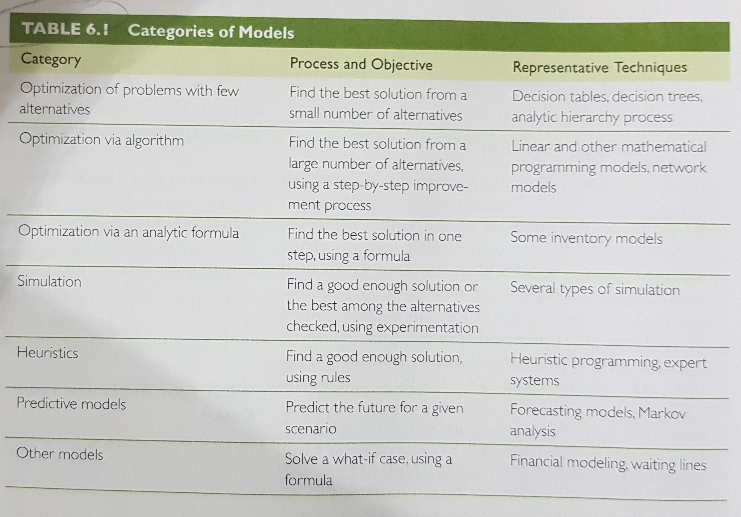
Categories of prescriptive models:

table 6.1

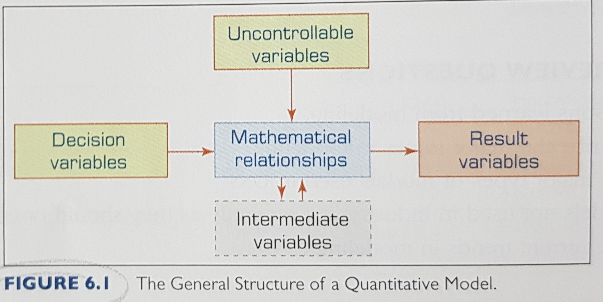
The general structure of a quantitave model:

figure 6.1

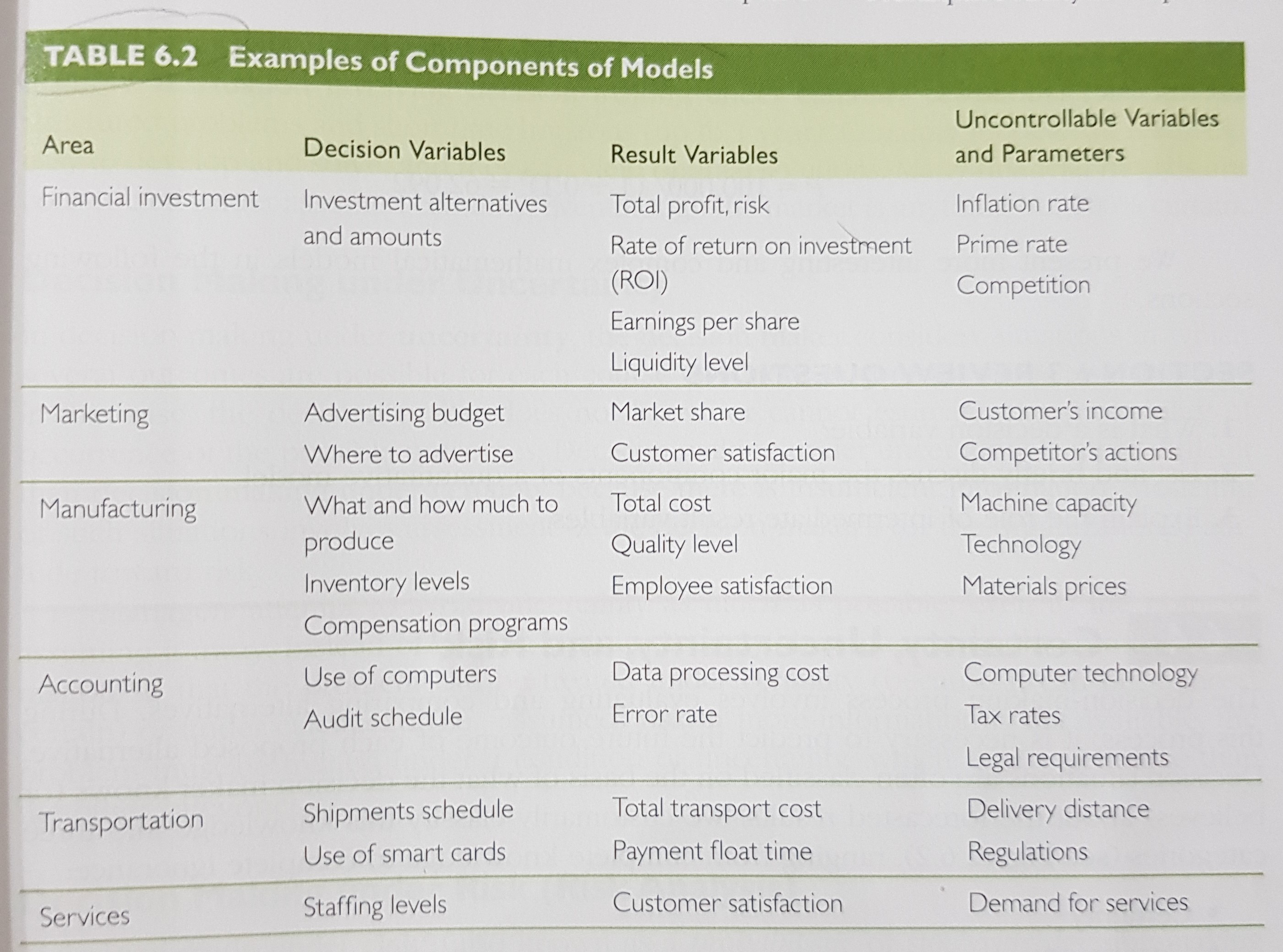
Some examples:

table 6.2

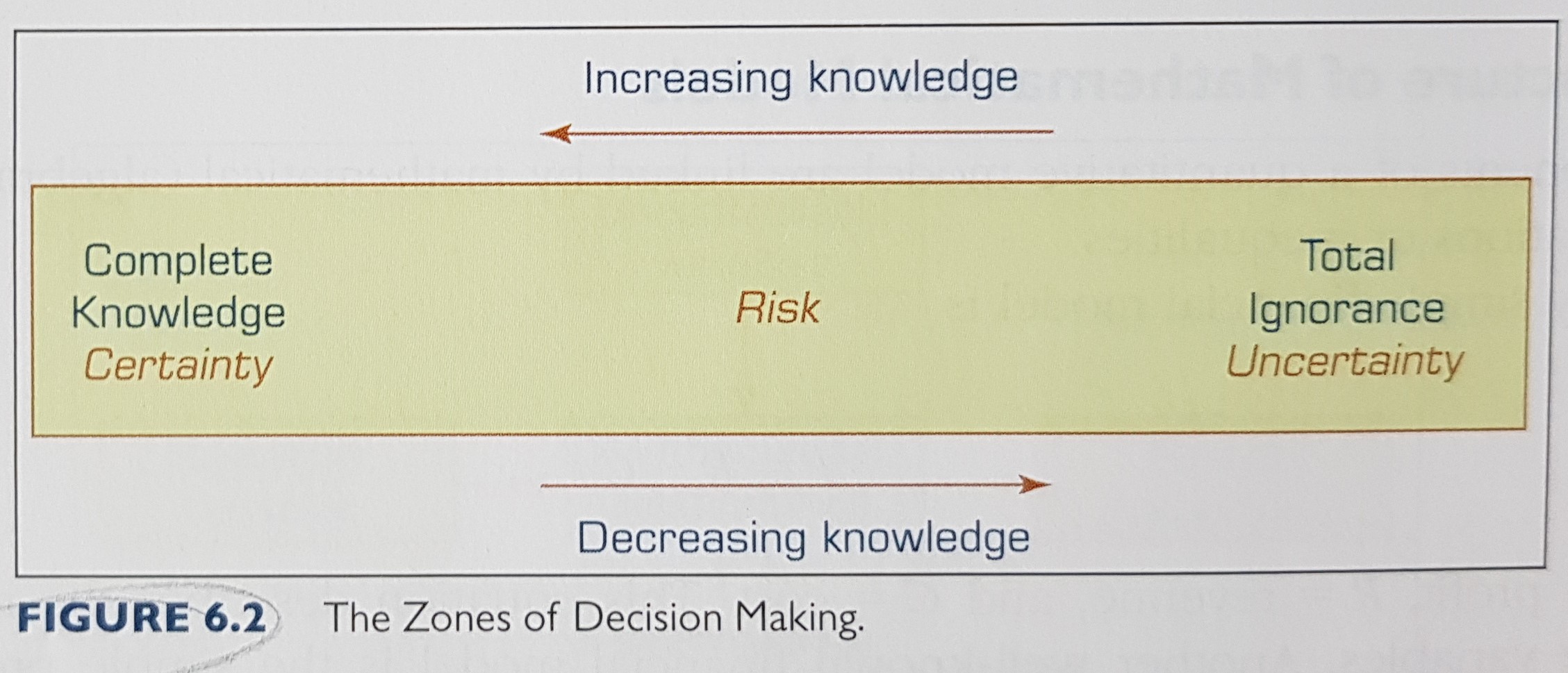
The zones of decision making:

figure 6.2

Characteristics of LP allocation problems:

a limited quantity of economic resources is available for allocation.
the resources are used in the production of products or services.
there are two or more ways in which the resources can be used, each is called a solution or a program.
each activity (product or service) in which the resources are used yields a return in terms of the stated goal.
the allocation is usually restricted by several limitations and requirements, called constraints.

The LP allocation model is based in the following rational economic assumptions:

returns from different allocations can be compared; that is, they can be measured by a common unit (e.g., dollars, utility).
the return from any allocation is independent of other allocations.
the total return is the sum of the returns yielded by the different activities.
all data are known with certainty.
the resources are to be used in the most economical manner.
usually many solutions are possible, but only one of them is optimal.

Composition of LP models:

decision variables – whose values are unknown and are searche for
objective function – a linear mathematical function that relates the decision variables to the goal, measures goal attainment, and is to be optimized.
objective function coeffecients – unit profit or cost coeffecients indicating the contribution to the objective of one unit of a decision variable.
constraints – expressed in the form of linear inequalities or equalities that limit resources and/or requirements; these relate the variables through linear relationships
capacities – which describe the upper and sometimes lower limits on the constraints and variables.
input/output technilogy coeffecients – which indicate resource utilization for a decision variable

Modeling in LP, an example:

figure 6.5

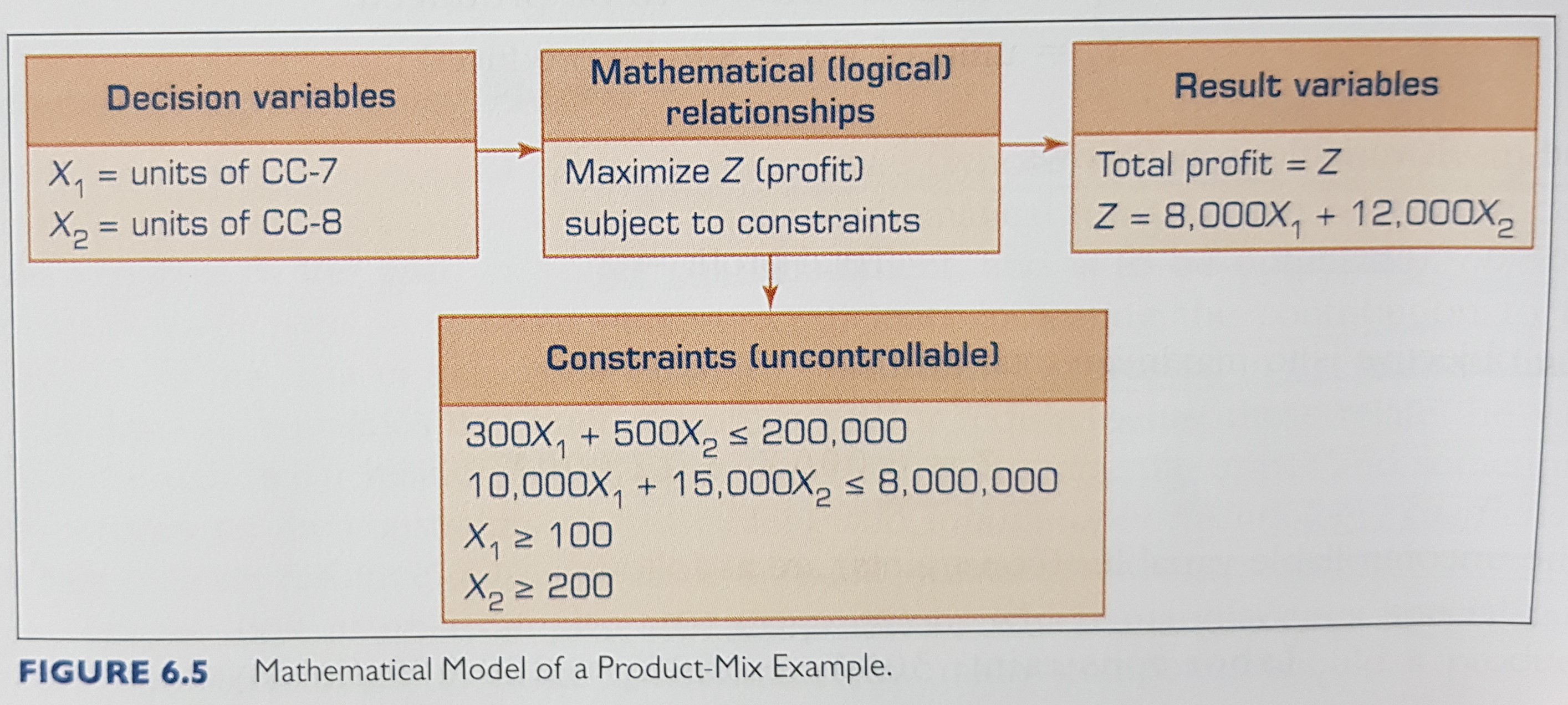
Notes:

Every LP model has some internal intermediate variables that are not explicitly stated. The labor and budget constraints may each have some slack in them when the left-hand side is strictly less than the right-hand side. this slack is represented internally by slack variables that indicate exces resources available.
In a real-world environment, it could possibly take months to obtain the data in the problem statement, and while gathering the data the decision maker would no doubt uncover facts about how to structure the model to be solved.

The most common optimization models can be solved by a variety of mathematical programming methods, including the following:

Certain difficulties may arise when analyzing multiple goals:

it is usually difficult to obtain an explicit statement of the organizations goals.
the decision maker may change the importance assigned to specific goals over time or for different decision scenarios.
goals and subgoals are viewed differently at various levels of the organization and within different departments.
goals change in response to changes in the organization and its environment.
the relationship between alternatives and their role in determining goal may be difficult to quantify.
complex problems are solved by groups of decision makers, each of whom has a personal agenda.
participants assess the importance (priorities) of the various goals differently.

Several methods of handling multiple goals can be used when working with such situations. the most common ones are:

Sensitivity analysis types:

automatic – it reports the range within which a certain input variable or parameter value (e.g., unit cost) can vary without having any significant impact on the proposed solution. automatic sensitivity analysis is usually limited to one change at a time, and only for certain variables.
trial-and-error – the impact of changes in any variable, or in several variables, can be determined through a simple trial-and-error approach.
- what-if analysis.
- goal seeking – calculates the values of the inputs necessary to achieve a desired level of an output (goal). it represents a backward solution approach. Can also be used to compute a break even point.

Strictly speaking, simulation is a descriptive rather than a prescriptive method. There is no automatic search for an optimal solution.
Simulation is a technique for conducting experiments.
Simulation is normally used only when a problem is too complex to be treated using numerical optimization techniques.

Some advantages of simulation:

a great aamount of time compression can be attained.
experimentation.
simplifications are not necessary, thus providing a wide range of possibilities.
handles relatively unstructured problems.

Some disadvantags:

The process of simulation:

figure 6.12

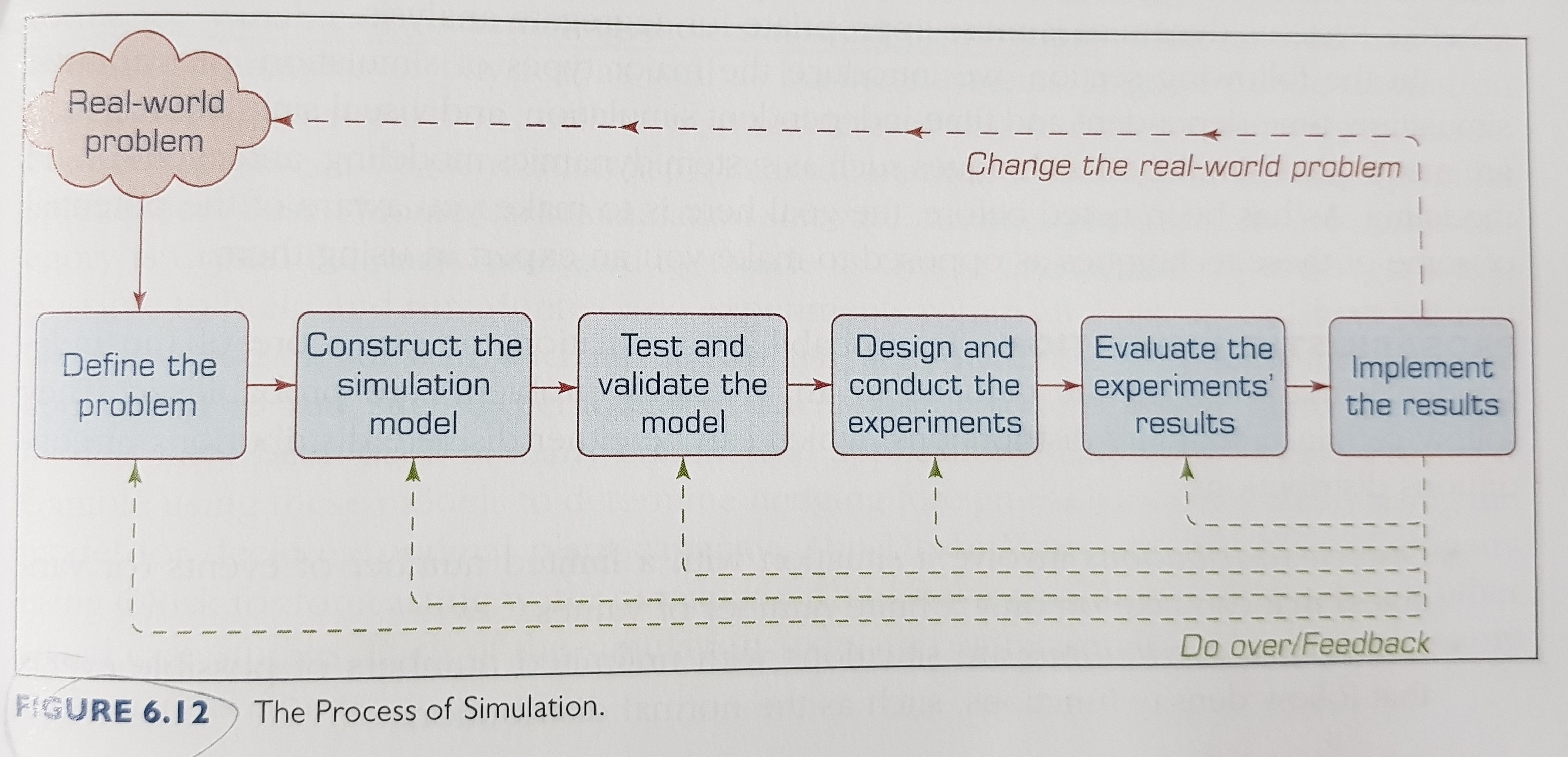
A popular type of simulation: monte carlo

This method usually begins with building a model of the decision problem without having to consider the uncertainty of any variables.
Then we recognize that certain parameters or variables are uncertain or follow an assumed or estimated probabilty distribution.
This estimation is based on analysis of past data.
Then we begin running sampling experiments.
These sampling experiments essentially amount to solving the same model many times.
We can then analyze the behaviour of these dependent variables by examining their statistical distributions.